Building a Two-Tower Deep Learning Movie Recommender System in Pytorch (from scratch)

Introduction
Recommender systems play a crucial role in content-serving websites such as TikTok, Amazon, Netflix, YouTube, etc, by effectively showing users relevant content. They also make these companies billions of dollars: 35% of Amazon.com’s revenue is generated by its recommendation engine.
What is a recommender system?
In my own words: a recommender system’s job is to match users to content. They score/rank which content to show based on some pre-determined metric to optimize (i.e. what content will the user find most relevant or engaging). Recommendation Systems exist because many platforms have thousands (or millions) of ‘things’ they could potentially show their users, and screen real estate is extremely valuable, so they help the platforms show only what they think the user will like. Without them, it would also be impossible for the user to sift through millions of options.
Use Cases
Recommender systems are used to decide:
- What movie to watch next on Netflix
- What product to buy next on Amazon
- What song to listen to next on Spotify
- What video to watch next on YouTube
- What post to watch next on Instagram feed
- What vacation to book next on Booking.com
Sneak Peek of this Post
Just to give an idea of what we are going to build here, it’s going to be a movie recommendation system that can give us recommendations for users like:
TLDR: Please follow this link to go straight to the Colab notebook with the PyTorch code discussed in this post.
Outline of this Post
- Introduction
- Why this Post
- Building a Movie Recommender
- Actually Using our Model
- Possible Improvements
- Appendix
Why this Post
There are already hundreds (probably thousands) of posts/tutorials/follow-alongs on ‘how to build a movie recommender system’. However, most of them are really really not useful. 90% of them just read in the dataset, perform cosine similarity on some vectors made out of the users and movies, show off some recommendations that make little sense, and call it a day. 10% will actually use Machine Learning, and of these, 90% will just do some variation of user-to-item matrix factorization and stop after they spit out some loss metrics (i.e. they won’t even show how it can be used).
Don’t get me wrong, MF is a great aproach to recommendation systems (I helped create a book recommendation system using it, and even helped write an entire CUDA library to parallelize it), but it’s not ‘state of the art’ anymore. The main drawback of basic MF is that does not incorporate rich user/item features in how it learns to predict ratings/interactions.
For even more information on MF, please look at these blog posts for a technical explanation of Matrix Factorization and an application of Matrix Factorization for book recommendation.
Deep Recommender Systems
The main approach I wanted to focus on is the ‘Two Tower’ Deep Learning Architecture. The idea is this: you want to recommend users to items (i.e. movies, products, songs, etc). You have features for users (what they have already watched/bought/clicked/etc, demographic information, etc.) and features for items (the genre of you movie/song, the artists/actors, the year, etc.). Can we shove all these features into a Neural Net and get good recommendations (hint: yes)?
There are some great tutorials on how to build modern day model architectures (including Two Tower models) to train a recommendation system model. Here is a list of a few of them:
- Scaling deep retrieval with TensorFlow Recommenders and Vertex AI Matching Engine
- Google: Build a Movie Recommendation System
- TFRS: Building deep retrieval models
- How to Implement a Recommendation System with Deep Learning and PyTorch
BUT: they all have serious a common serious drawback: NONE show you how to ‘actually’ use these things. It’s all ‘left to the reader as an exercise.’
The Core Issue
All of the above examples (and others I could find) use the traditional approach of embedding the unique user ids (or hashes of something unique like a username) and movie ids (like an Amazon product id) to train the model. However, this means that you can ONLY perform inference for a user or item that has been trained. If you want to run inference on a user id that you did not train on, you won’t have an embedding for them and are out of luck. If a new user wanted to use this model, your only solutions are:
- Retrain the entire model
- Try to partial fit your new user into the model with some training steps
- Find a user that is close to the new user and use their embedding
The Goal
Instead, I wanted to set out to build a model that can generalize to any user, as long as you provide even a few examples of items they alreay enjoyed (i.e. when you sign up to Nick-flix Movie Streaming, you click on a few movies you like). The model should embed features of the user, not the unique user themselves. This is different than most other tutorials in that we will NOT map each user id to an embedding. Instead, for our simple example, we will treat each user as a feature vector made up of only two pieces of information:
- Their Watch History: list of movies they have liked/disliked
- Their Genre Preferences: the average rating for each possible genre
This way, after the model is trained, it can be used to get recommendations for any user as long as we have even a few movies they like (maybe some genres they prefer or don’t prefer).
Benefits
There are a few benefits to this approach:
- Do not need to retrain model as often
- Model is more generalizable as it cannot just memorize labels for specific users
- User level cold start is much less of an issue
A Note about Item Cold Start
Removing the user id from the model helps generalize to more users, and also reduces user cold start. But what about item cold start (new item, so no item id in the model)? To get around this, it’s also possible to remove the item id from the model input and only use item features as inputs.
This post does a great job explaining how having NO ids helps with cold start: Solving the Cold-Start Problem using Two-Tower Neural Networks for NVIDIA’s E-Mail Recommender Systems
As with all things, there are tradeoffs. By removing the item id, you will lose a lot of rich information about how users interact with unique items. However, you massively reduce cold start.
Some domains might be better or worse to keep or remove ids: Amazon has millions of products and probably thousands added each day that need to be recommended. They could benefit from removing unique item ids from their models. Netflix, on the other hand, might only have a few dozen movies added per month to their catalog. They might want to keep the movie id and retrain their model more frequently.
Another possibility is to train a normal model with id embeddings, and then a second model with just features. You can then mix and match the results of both.
Building a Movie Recommender
Alright, let’s start building our recommendation system!
The Dataset
In order to build a Movie recommendation system, we are going to use the MovieLens Dataset which is provided by GroupLens
In particular, we are going to use two datasets, one small and one large:
- MovieLens Small - 100,000 ratings, 9,000 movies, 600 users.
- MovieLens Latest - 33,000,000 ratings, 86,000 movies, 330,975 users.
The small dataset does not lead to good results, but it is better to use while building and testing our code.
We can read in this data as a Pandas Dataframe easily like this:
df_ratings = pd.read_csv('ratings.csv')
df_movies = pd.read_csv('movies.csv')
The data will consists of two Pandas Dataframes we will read in:
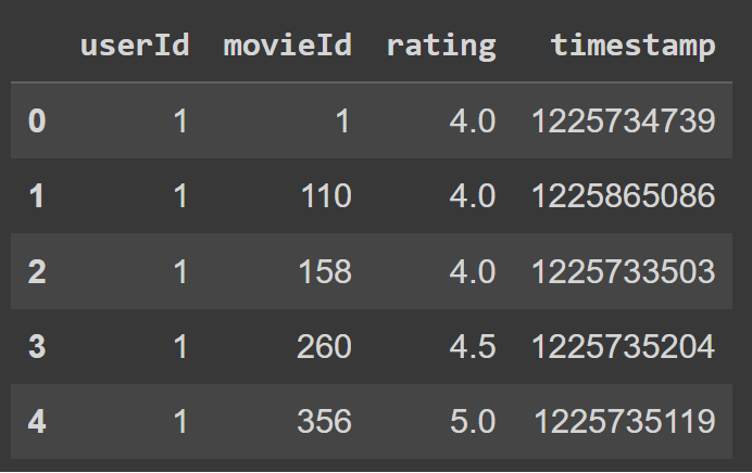 |
|---|
| Ratings Table |
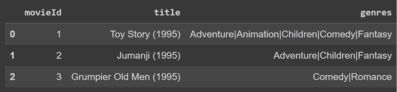 |
|---|
| Movies Table |
Data Preprocessing
First, we need to clean the data as any ‘nan’ values can completely ruin our training (I spent many hours debugging my model, adding gradient clipping, batch norm, etc. Turns out there is a single nan value in MovieLens). We also convert movie ids to ints so they behave better as lookup keys.
# clean the ratings data
df_ratings = df_ratings.dropna()
df_ratings['movieId'] = df_ratings['movieId'].astype(int, copy=False)
Next, let’s shrink down how many movies we care about.
NOTE: This is just for memory reasons. Google colab only gives you 12GB of RAM, so I can’t createa embeddings and feature vectors for all 50k+ movies.
# let's only work with movies with enough ratings.
min_ratings_per_movie = 1000

# get the number of ratings per movie
df_movies_to_num_ratings = df_ratings.groupby('movieId', as_index=False)['rating'].count()
print("total movies in corpus: ", len(df_movies_to_num_ratings))

df_movies_to_num_ratings = df_movies_to_num_ratings.sort_values(by=['rating'], ascending=False)
df_movies_to_num_ratings = df_movies_to_num_ratings[df_movies_to_num_ratings['rating'] > min_ratings_per_movie]
print("movies with enough ratings: ", len(df_movies_to_num_ratings))

# get list of the top movies by number of ratings.
top_movies = df_movies_to_num_ratings.movieId.tolist()

# OUTPUT
# total movies in corpus:  58136
# movies with enough ratings:  2071
Movie Feature Preprocessing
Let’s start processing some important info we need for our movies.
First, let’s create a simple map to hold how many ratings each movie has.
# keep a map of movieId to number of ratings.
movieId_to_num_ratings = {}
movieId_list = df_movies_to_num_ratings.movieId.tolist()
rating_list = df_movies_to_num_ratings.rating.tolist()
for i in range(len(movieId_list)):
  movieId_to_num_ratings[movieId_list[i]] = rating_list[i]
Next, we reduce our Ratings Dataframe to get rid of any movies we don’t care about.
# reduce our df_ratings Dataframe to only rows that are top movie (to speed up later cells).
df_ratings_final = df_ratings[df_ratings.movieId.isin(top_movies)]
Next, let’s make a helpful map from each movie id to it’s title.
# map movieId to title
movieId_to_title = {}
title_to_movieId = {}

movieId_list = df_movies.movieId.tolist()
title_list = df_movies.title.tolist()

for i in range(len(movieId_list)):
  movieId = movieId_list[i]
  title = title_list[i]

  movieId_to_title[movieId] = title
  title_to_movieId[title] = movieId
Let’s take a look at our top movies
for movieId in top_movies[0:10]:
  print(movieId, movieId_to_title[movieId], movieId_to_num_ratings[movieId])
| movieId | title | num_ratings |
|---|---|---|
| 318 | Shawshank Redemption, The (1994) | 36414 |
| 356 | Forrest Gump (1994) | 33846 |
| 296 | Pulp Fiction (1994) | 32440 |
| 2571 | Matrix, The (1999) | 31830 |
| 593 | Silence of the Lambs, The (1991) | 30452 |
Next, let’s map each movie to a set() of its genres. These will be used as item features for our model (i.e. a movie will be represented as a vector of its genre information).
# map movieId to list of genres for that movie
genres = set()
movieId_to_genres = {}

movieId_list = df_movies.movieId.tolist()
genre_list = df_movies.genres.tolist()

for i in range(len(movieId_list)):
  movieId = movieId_list[i]
  if movieId not in top_movies:
    continue

  movieId_to_genres[movieId] = set()

  for genre in genre_list[i].split('|'):
    genres.add(genre)
    movieId_to_genres[movieId].add(genre)
Let’s print out an example of a movie’s genres:
print(movieId_to_genres[title_to_movieId['Matrix, The (1999)']])
# OUTUPT: {'Action', 'Sci-Fi', 'Thriller'}
Next, let’s get the average rating of every movie. This is helpful later as we want to make sure our model isn’t just recommending the most popular movies.
# for every movie, get the avg rating
df_movies_to_avg_rating = df_ratings_final.groupby('movieId', as_index=False)['rating'].mean()

movieId_to_avg_rating = {}

movieId_list = df_movies_to_avg_rating.movieId.tolist()
rating_list = df_movies_to_avg_rating.rating.tolist()
for i in range(len(movieId_list)):
  movieId_to_avg_rating[movieId_list[i]] = rating_list[i]
Movie Feature Vocab
This is a pretty important part of the data prep. Setting up a feature vocab is needed to correctly map movie ids and movie features (i.e. only genres in our case) to the correct indices in input feature vectors.
Below, we map each unique movie id we have in top_movies to a unique index i. This will allow us to look up this movie’s embedding efficiently.
# build ITEM movieId embedding mapping
item_emb_movieId_to_i = {s:i for i,s in enumerate(top_movies)}
item_emb_i_to_movieId = {i:s for s,i in item_emb_movieId_to_i.items()}
Below, we map each unique genre to an index i that will be used to set each moveie’s genres in vector form. For example, if we had 3 genres, ‘Action’, ‘Horror’, and ‘Comedy’, we could map ‘Action’ to index 0, ‘Horror’ to index 1, and ‘Comedy’ to index 2. Therefore, and genre vector representation of movie that is an ‘Action Comedy’ movie would be [1, 0, 1].
# build ITEM genre feature context
genre_to_i = {s:i for i,s in enumerate(genres)}
i_to_genre = {i:s for s,i in genre_to_i.items()}
User Feature Preprocessing
Every user will have a feature context that will mostly be their watch history. Instead of using every movie in the corpus, we can use a smaller subset. This also helps with memory issues.
num_movies_for_user_context = 250
user_context_movies = top_movies[:num_movies_for_user_context]
Next, let’s simplify our Ratings dataframe so we can much more efficiently iterate over it and create training examples.
# aggregate dataframe down into one row per user and list of their movies and ratings.
df_ratings_aggregated = df_ratings_final.groupby('userId').agg({'movieId': lambda x: list(x), 'rating': lambda y: list(y)}).reset_index()
The above code looks complicated, but actually all it is doing is finding all the rows where a userId equals a unique value, and collapsing all the values in the movieId and rating column into a list. We do this because dataframes are extremely inefficient to iterate over. We need to do this aggregation to get all the ratings for a user, so the more we can do inplace in the Dataframe, the better.
The Dataframe now looks like this (and has one row per user):
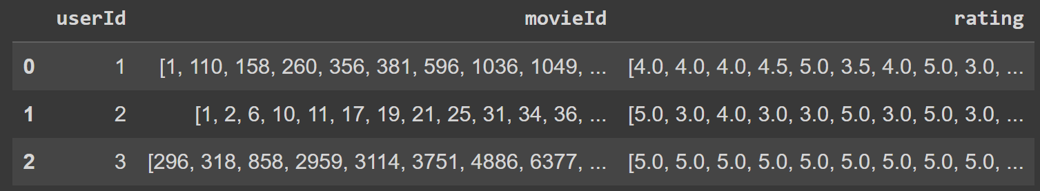 |
|---|
| Aggregated Ratings Table |
User Feature Vocab
Our user vocab will be slighly different than our movie vocab. This is because we actually will ignore the userId and not use it to look up some predefiend embedding. Instead, we will map every user to a feature vector that is made up of two parts
- The movies the user has already watched
- The avg rating per genre for this user (think of this as the user’s preferences)
This means it is entirely possible that two unique users have the same feature vector representation.
# build the USER context
user_context_size = len(user_context_movies) + len(genres)

user_context_movieId_to_i = {s:i for i,s in enumerate(list(user_context_movies))}
user_context_i_to_movieId = {i:s for s,i in user_context_movieId_to_i.items()}

user_context_genre_to_i = {s:i+len(user_context_movies) for i,s in enumerate(list(genres))}
user_context_i_to_genre = {i:s for s,i in user_context_genre_to_i.items()}
The full feature vector for a user will be one vector which is a concatanation of their watch history and their genre preferences. Let’s assume we have 3 movies and 3 genres.
- Movies: Movie1, Movie2, Movie3
- Genres: Action, Horror, and Comedy
For a user that liked Movie1 and disliked Movie3, and likes Action and Comedy but hates Horror, their feature vector would look like:
['movie1', 'movie2', 'movie3', 'action', 'horror', 'comedy']
[     1.0,      0.0,     -1.0,      1.0,     -1.0,      1.0]
Generating Training Examples
Next, we simulate real world training examples by masking out some of the user’s watched movies from their context, and using them as labels. We do not want the ‘movie to predict’ in their watch history, as we are trying to simulate the following: given the user’s other watched movies, what would they rate this new movie?
NOTE: this is not the same as a train/test split. This is just simulating how training examples would look like on a movie platform.
WARNING: In the real world, as a user watches movies organically, you’d build up their watch history naturally and train a model using their older watch history to predict their most recent watches. If we wanted to be more correct, we could sort our ratings by timestamp and use older watches to predict newer watches, but it’s not necessary for the sake of this tutorial.
percent_ratings_as_watch_history = 0.8

user_to_movie_to_rating_WATCH_HISTORY = {}
user_to_movie_to_rating_LABEL = {}

# loop over each column as this is much, much faster than going row by row.
user_list = df_ratings_aggregated['userId'].tolist()
movieId_list_list = df_ratings_aggregated['movieId'].tolist()
rating_list_list = df_ratings_aggregated['rating'].tolist()

for i in range(len(user_list)):
  userId = user_list[i]
  movieId_list = movieId_list_list[i]
  rating_list = rating_list_list[i]

  num_rated_movies = len(movieId_list)

  # ignore users with too few ratings.
  if num_rated_movies <= 5: continue

  # set up training example maps.
  user_to_movie_to_rating_WATCH_HISTORY[userId] = {}
  user_to_movie_to_rating_LABEL[userId] = {}

  # shuffle the user's movies that they have watched
  rated_movies = list(zip(movieId_list, rating_list))
  random.shuffle(rated_movies)

  # put some movies into user's watch history (features) and leave others as labels to predict.
  for movieId,rating in rated_movies[:int(num_rated_movies * percent_ratings_as_watch_history)]:
    user_to_movie_to_rating_WATCH_HISTORY[userId][movieId] = rating
  for movieId,rating in rated_movies[int(num_rated_movies * percent_ratings_as_watch_history):]:
    user_to_movie_to_rating_LABEL[userId][movieId] = rating
Set up Feature Vectors
First, we need each user’s average rating. This is so we can de-bias each rating. If the user’s rating is above their average for a movie, we will treat that as a positive value in their vector. Opposite for ratings below their average. This helps the model learn likes and dislikes.
user_to_avg_rating = {}

# NOTE: only use ratings from their synthetic watch history.
for user in user_to_movie_to_rating_WATCH_HISTORY.keys():
  user_to_avg_rating[user] = 0
  for movieId in user_to_movie_to_rating_WATCH_HISTORY[user].keys():
    user_to_avg_rating[user] += user_to_movie_to_rating_WATCH_HISTORY[user][movieId]

  user_to_avg_rating[user] /= len(user_to_movie_to_rating_WATCH_HISTORY[user].keys())
Next, let’s get each user’s preference for each genre. We will compute the user’s average rating for each genre and de-bias it.
# for every user, get the avg rating for every genre
user_to_genre_to_stat = {}

# NOTE: only use ratings from their synthetic watch history.
for user in user_to_movie_to_rating_WATCH_HISTORY.keys():
  user_to_genre_to_stat[user] = {}
  for movieId in user_to_movie_to_rating_WATCH_HISTORY[user].keys():
    for genre in movieId_to_genres[movieId]:
      if genre not in user_to_genre_to_stat[user]:
        user_to_genre_to_stat[user][genre] = {
            'NUM_RATINGS': 0,
            'SUM_RATINGS': 0,
        }

      user_to_genre_to_stat[user][genre]['NUM_RATINGS'] += 1
      user_to_genre_to_stat[user][genre]['SUM_RATINGS'] += user_to_movie_to_rating_WATCH_HISTORY[user][movieId]

for user in user_to_genre_to_stat.keys():
  for genre in user_to_genre_to_stat[user].keys():
    num_ratings = user_to_genre_to_stat[user][genre]['NUM_RATINGS']
    sum_ratings = user_to_genre_to_stat[user][genre]['SUM_RATINGS']
    user_to_genre_to_stat[user][genre]['AVG_RATING'] = sum_ratings / num_ratings
Finaly, we can build a feature ‘context’ vector for every user using their watch history and genre preferences.
# for every user, create the training example user context vector
# 0:num_user_context_movies -> user's watch history
# num_user_context_movies:num_user_context_movies+num_genres -> user's genre affinity
user_to_context = {}
for user in user_to_movie_to_rating_WATCH_HISTORY.keys():
  context = [0.0] * user_context_size

  for movieId in user_to_movie_to_rating_WATCH_HISTORY[user].keys():
    if movieId in user_context_movies:
      # note, we debias the rating so if the rating is under the user's avg rating,
      # it will hopefully count as negative strength for predicting similar movies.
      # vice-versa for a rating above the user's average.
      context[user_context_movieId_to_i[movieId]] = float(user_to_movie_to_rating_WATCH_HISTORY[user][movieId] - user_to_avg_rating[user])

  for genre in user_to_genre_to_stat[user].keys():
    context[user_context_genre_to_i[genre]] = float(user_to_genre_to_stat[user][genre]['AVG_RATING'] - user_to_avg_rating[user])

  user_to_context[user] = context
We also need to set up the feature vector for each movie. This is much simpler since it’s just a binary mask vector for every genre the movie has.
# for every movie, create a training example feature context vector lookup
# it will contain the movie's genres.
movieId_to_context = {}
for movieId in top_movies:
  context = [0.0] * len(genres)

  for genre in movieId_to_genres[movieId]:
    context[genre_to_i[genre]] = float(1.0)

  movieId_to_context[movieId] = context
Designing our Model Architecture
Before we build the final dataset, it would be helpful to know why it will be the way it is. Unlike most datasets you might have seen with just an X and Y matrix to hold inputs and labels, we are building a Two Tower model (technically it has 3 inputs).
Here is our model and I’ll explain it in detail.
'''
user_features ---------------> u_W1
                                    \
                                     \
                                      --> dot_product(user, item) --> prediction
                                     /
movie_features  -> i_W1             /
                        \          /
                         --> stack
                        /
movie_embedding -> e_W1
'''
Our model will have 3 inputs that each feed into a non-linear layer.
- The user’s context feature vector
- The movie’s context feature vector
- The movie’s id embedding vector
The final output is a prediction for the user’s rating for the movie. This prediction is based on the user’s feeatures, the movie’s features, and the learned embedding for the unique movie id.
To get the prediction, we concatanate the hidden embeddings from both movie inputs, and compute the dot product with the ‘combined movie embedding vector’ and the ‘user embedding vector’.
We will train this model by simply computing the loss of the actual user’s rating for this movie versus the predicted loss.
Backpropogation works normally even for this ‘Two Tower’ model.
Building our Dataset
Now that you understand the inputs and output of our model, let’s actually build the Dataset. It consists of 4 parts:
- The user context feature vectors, held in matrix X
- The target movie’s id, held in vector target_movieId
- The target movie’s context feature vectors, held in matrix target_movieId_context
- The target movie’s actual rating, held in vector Y
Each part of the Dataset will be converted to a Pytorch Tensor so it can be used in Pytorch funtions to feed and train the model.
# Build the final Dataset
def build_dataset(users):
  # the user context (i.e. the watch hisotyr and genre affinities)
  X = []

  # the movieID for the movie we will predict rating for.
  # used to lookup the movie embedding to feed into the NN item tower.
  target_movieId = []

  # the feature context of the movie we will predict the rating for.
  # will also feed into it's own embedding and will be stacked with the embedding above.
  target_movieId_context = []

  # the predicted rating
  Y = []

  # create training examples, one for each movie the user has that we want as a label.
  for user in users:
    for movieId in user_to_movie_to_rating_LABEL[user].keys():
      X.append(user_to_context[user])

      target_movieId.append(item_emb_movieId_to_i[movieId])

      target_movieId_context.append(movieId_to_context[movieId])

      # remember to debias the user rating so we can learn to predict if user
      # like/dislike a movie based on their features and the movie features.
      Y.append(float(user_to_movie_to_rating_LABEL[user][movieId] - user_to_avg_rating[user]))

  X = torch.tensor(X)
  Y = torch.tensor(Y)
  target_movieId = torch.tensor(target_movieId)
  target_movieId_context = torch.tensor(target_movieId_context)

  return X,Y,target_movieId,target_movieId_context
Train/Validation Split
Before we call the build_dataset function, let’s split up some users into Train and some users into Validation.
WARNING: It would be more correct to shuffle the Dataset and include some training examples into our training set and others into validation set. But for the simplicity of this example, I will simply use some users for training and some for validation.
# user users with enough ratings to predict to be useful for model learning.
final_users = []

for user in user_to_movie_to_rating_LABEL.keys():
  num_ratings = len(user_to_movie_to_rating_LABEL[user])

  if num_ratings >= 2 and num_ratings < 500:
    final_users.append(user)
# split users into train and validation users
percent_users_train = 0.8

random.shuffle(final_users)

train_users = final_users[:int(len(final_users) * percent_users_train)]
validation_users = final_users[int(len(final_users) * percent_users_train):]
Finally, let’s get our training and valadation Datasets.
X_train, Y_train, target_movieId_train, target_movieId_context_train = build_dataset(train_users)
X_val, Y_val, target_movieId_val, target_movieId_context_val = build_dataset(validation_users)
Building our Model
Below, we will actually build from scratch the entire model (i.e. all the weights and biases). Notice the input dimensions of each of the parts. Each weight matrix links up to one of our inputs. i_W1 will match the dimensions of the movie feature vector, which is the number of genres. e_W1 is any size we want since we are creating an ITEM_EMBEDDING_LOOKUP. If this concept is confusing, please see Andrej Karpathy’s amazing series: Neural Networks: Zero to Hero.
NOTE: using an embedding lookup table is no different than simply creating a one-hot encoded vector of size len(top_movies) and just multiplying it by some matrix. However, that way is extremely inefficient and I was unable to train any decently sized model due to RAM constraints.
Few other small points:
- I scale the weights down a little to prevent early training iterations having crazy loss. If this was an actual production model, I’d probably apply BatchNorm on it.
- I’m using MSELoss which means we will get the average ‘Squared Error’ loss on all examples. This just means we square the difference of the real rating vs the predicted rating.
- We set a batch size of 64.
- I create two lists to hold our loss for our full training set and validation set. We will plot this later.
g = torch.Generator().manual_seed(42)

# ITEM movie feature tower
item_feature_embedding_size = 25
i_W1 = torch.randn((len(genres), item_feature_embedding_size), generator=g)
i_b1 = torch.randn(item_feature_embedding_size, generator=g)

# ITEM movie embedding tower
item_movieId_embedding_size = 25
ITEM_EMBEDDING_LOOKUP = torch.rand((len(top_movies), item_movieId_embedding_size), generator=g)
e_W1 = torch.randn((item_movieId_embedding_size, item_movieId_embedding_size), generator=g)
e_b1 = torch.randn(item_movieId_embedding_size, generator=g)

# USER feature tower
user_feature_embedding_size = 50 # must be the concat dimension of both item embeddings.
u_W1 = torch.randn((user_context_size, user_feature_embedding_size), generator=g)
u_b1 = torch.randn(user_feature_embedding_size, generator=g)

# create a list of all our TRAINABLE params
parameters = [
    i_W1, i_b1,
    ITEM_EMBEDDING_LOOKUP, e_W1, e_b1,
    u_W1, u_b1,
]

# normalize the initial weight values.
weight_scale = 0.1
for p in parameters:
  p *= weight_scale

# set all parameters to require gradients
for p in parameters:
  p.requires_grad = True

# print number of trainable params in our NN
print(sum(p.nelement() for p in parameters))

# set the loss function we want to use.
# we use MSE Loss because we are predicting the rating per label movie.
loss = torch.nn.MSELoss()

# set how big we want each minibatch to be
minibatch_size = 64

# create list to hold our loss per training iterations
loss_train = []
loss_val = []
Training our Model
Below is the actual code to train our model without the use of any Pytorch library. I write this all out manually versus using a Torch Module so we can control and study every single part and really understand each step.
Some notes:
- Every 1000 iterations, we will compute our loss on the full validation set.
- If we are doing a validation run, we will not backprop (won’t train)
- If we are doing a full validation run, we will use our validation Dataset pieces.
- torch.einsum is how we will do batched dot products of our user and movie embeddings to get the final prediction.
- We will gradually decrease our learning rate. We could use an optimizer, but I wanted to avoid Torch libraries.
- We record our avg loss during training and for each full validation runs.
log_every = 1000

for i in range(0, 50_000):

  # every so often, let's train and compute loss on entire validation set
  is_full_val_run = False
  if i % log_every == 0:
    is_full_val_run = True

  # select training example inputs we use for this run, and minibatch indices.
  X = X_train
  Y = Y_train
  target_movieId_context = target_movieId_context_train
  target_movieId = target_movieId_train
  if is_full_val_run:
    X = X_val
    Y = Y_val
    target_movieId_context = target_movieId_context_val
    target_movieId = target_movieId_val

  # construct a minibatch
  ix = torch.randint(0, X.shape[0], (minibatch_size,))
  if is_full_val_run:
    ix = torch.randint(0, X.shape[0], (X.shape[0],))

  # ---------- FORWARD PASS ----------

  # forward the USER tower.
  user_contexts = X[ix]
  user_embedding = torch.tanh(user_contexts @ u_W1 + u_b1)

  # forward the ITEM movie feature tower
  movie_contexts = target_movieId_context[ix]
  item_feature_embedding = torch.tanh(movie_contexts @ i_W1 + i_b1)

  # lookup the ITEM movieId embedding and pass through non-linear layer.
  # NOTE: this is just a shortcut to multiplying a one-hot vector with the masked movieID with a weight matrix.
  item_embedding_hidden = torch.tanh(ITEM_EMBEDDING_LOOKUP[target_movieId[ix]] @ e_W1 + e_b1)

  # concat/stack the two ITEM embeddings together
  item_embedding_combined = torch.cat((item_feature_embedding.view(item_feature_embedding.size(0), -1),
                                       item_embedding_hidden.view(item_embedding_hidden.size(0), -1)), dim=1)

  # the final prediction is the dot product of the user embedding and the combined item embedding.
  # NOTE: because we have a batch of these, we will use torch.einsum to do this efficiently.
  preds = torch.einsum('ij, ij -> i', user_embedding, item_embedding_combined)

  # compute the loss of our predicted ratings
  output = loss(preds, Y[ix])

  # backpropogation and update weights (except on validation runs)
  if not is_full_val_run:
    for p in parameters:
      p.grad = None

    output.backward()

    # update weights using gradients * learning_rate
    lr = 0.1
    if i >= 10_000: lr = 0.05
    if i >= 20_000: lr = 0.01
    if i >= 30_000: lr = 0.005
    for p in parameters:
      p.data += (lr * -p.grad)

  # every so often, log the MSE loss on full val set (see above)
  if is_full_val_run:
    loss_val.append(output.item())

    if i >= log_every:
      avg_train_loss_last_batches = np.mean(loss_train[i-log_every:i])
    else:
      avg_train_loss_last_batches = output.item()
    print("[TRAIN] i: ", i, " | ", "loss: ", avg_train_loss_last_batches)
    print("[VAL] i: ", i, " | ", "loss: ", output.item())
    print()
  else:
    loss_train.append(output.item())
As the model trains, we should see something liks this being printed:
[TRAIN] i:  0  |  loss:  0.9906623363494873
[VAL] i:  0  |  loss:  1.0060031414031982

[TRAIN] i:  1000  |  loss:  0.8815735578536987
[VAL] i:  1000  |  loss:  0.896892786026001

[TRAIN] i:  2000  |  loss:  0.8524652123451233
[VAL] i:  2000  |  loss:  0.8721503019332886
Finally, we can plot our training and validation losses versus each iteration.
loss_train_bucket_means = []
for i in range(0, len(loss_train), log_every):
  loss_train_bucket_means.append(np.mean(loss_train[i:i+log_every]))

plt.plot([i*1000 for i in range(len(loss_train_bucket_means))], loss_train_bucket_means)
plt.plot([i*1000 for i in range(1, len(loss_val))], loss_val[1:])
It will look something like this:
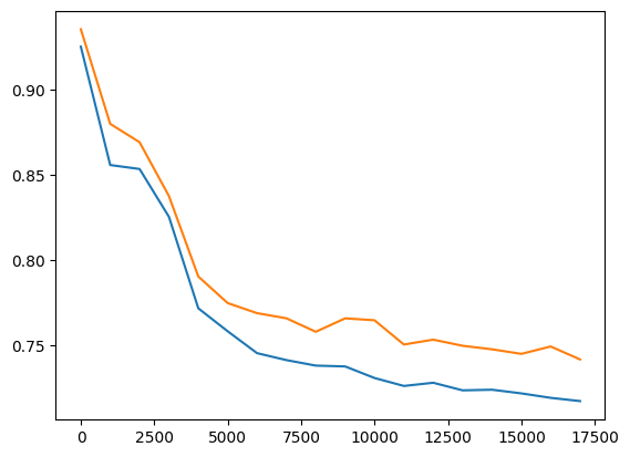 |
|---|
| Example train vs val loss plot |
Actually Using our Model
Now for the fun part: let’s actually use this trained model to generate recommendations for different types of users we might see (if we were Netflix for example).
Precomputing Movie Embeddings
In oder to get recommendations, we will feed in a new user feature vector through our model, and get a predicted rating for every movie in top_movies. To get a prediction for a movie, we need the item embedding in order to do the dot product with the user embedding. For different users, we don’t need to recompute these embeddings: once we have them for every movie in our catalog, we can re-use them!
We can compute our final embeddings for every movie all at once, then save them to a lookup map, and then easily use them later for any user (no need to ever do a forward pass in the Item Tower).
# for every movie, save all its embeddings
movieId_to_embedding = {}

for movieId in top_movies:
  movieId_to_embedding[movieId] = {}

  item_embedding = ITEM_EMBEDDING_LOOKUP[torch.tensor([item_emb_movieId_to_i[movieId]])]
  movieId_to_embedding[movieId]['MOVIEID_EMBEDDING'] = torch.tanh(item_embedding @ e_W1 + e_b1)

  movieId_to_embedding[movieId]['MOVIE_FEATURE_EMBEDDING'] = torch.tanh(torch.tensor([movieId_to_context[movieId]]) @ i_W1 + i_b1)

  # compute the combined (concat) item/movie embedding
  item_id_emb = movieId_to_embedding[movieId]['MOVIEID_EMBEDDING']
  item_feature_emb = movieId_to_embedding[movieId]['MOVIE_FEATURE_EMBEDDING']
  movieId_to_embedding[movieId]['MOVIE_EMBEDDING_COMBINED'] = torch.cat((item_feature_emb.view(item_feature_emb.size(0), -1),
                                       item_id_emb.view(item_id_emb.size(0), -1)), dim=1)
Finding Most Similar Movies
Since we now have a vector representation of every movie, we can easily find each movie’s most similar movies. This can be useful by itself and companies like Amazon use similar embeddings to power things like ‘Similar to What you just Bought’.
# for every movie, and for every embedding type, find the similary to all other embeddings
# NOTE: can be slow
movieId_to_emb_type_to_similarities = {}

for movieId in top_movies:
  movieId_to_emb_type_to_similarities[movieId] = {}

  for emb_type in movieId_to_embedding[movieId].keys():
    emb_to_target_to_dist = {}
    for target_id in top_movies:
      src = movieId_to_embedding[movieId][emb_type].view(-1)
      target = movieId_to_embedding[target_id][emb_type].view(-1)

      distance = torch.sqrt(torch.sum(torch.pow(torch.subtract(src, target), 2), dim=0))
      emb_to_target_to_dist[target_id] = distance.item()
    movieId_to_emb_type_to_similarities[movieId][emb_type] = sorted(emb_to_target_to_dist.items(), key=lambda item: item[1])
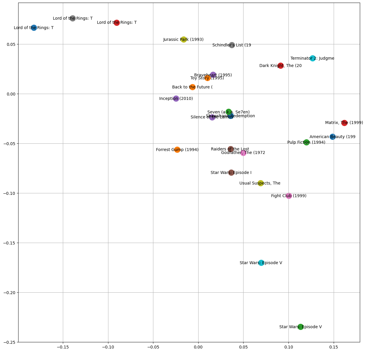
Most Similar to: Lord of the Rings: The Return of the King, The (2003)
Lord of the Rings: The Fellowship of the Ring, The (2001)
Lord of the Rings: The Two Towers, The (2002)
Hobbit: An Unexpected Journey, The (2012)
Gladiator (2000)
Dune (2021)
Most Similar to: Star Wars: Episode IV - A New Hope (1977)
Star Wars: Episode V - The Empire Strikes Back (1980)
Star Wars: Episode VI - Return of the Jedi (1983)
Raiders of the Lost Ark (Indiana Jones and the Raiders of the Lost Ark) (1981)
Indiana Jones and the Last Crusade (1989)
Ghostbusters (a.k.a. Ghost Busters) (1984)
Most Similar to: Toy Story (1995)
Toy Story 2 (1999)
Toy Story 3 (2010)
Monsters, Inc. (2001)
Inside Out (2015)
Bug's Life, A (1998)
Most Similar to: Saving Private Ryan (1998)
Braveheart (1995)
Black Hawk Down (2001)
Last of the Mohicans, The (1992)
Untouchables, The (1987)
Dirty Dozen, The (1967)
Most Similar to: Kill Bill: Vol. 1 (2003)
Ronin (1998)
French Connection, The (1971)
Run Lola Run (Lola rennt) (1998)
Sin City (2005)
Fistful of Dollars, A (Per un pugno di dollari) (1964)
Most Similar to: American Pie (1999)
American Pie 2 (2001)
Liar Liar (1997)
Wedding Singer, The (1998)
Meet the Parents (2000)
Wedding Crashers (2005)
Most Similar to: Princess Mononoke (Mononoke-hime) (1997)
Spirited Away (Sen to Chihiro no kamikakushi) (2001)
Howl's Moving Castle (Hauru no ugoku shiro) (2004)
Spider-Man: Into the Spider-Verse (2018)
Akira (1988)
Ghost in the Shell (Kôkaku kidôtai) (1995)
Inference: Getting Recommendations
Now for the best part: let’s actually get some recommendations for different types of movie lovers!
To get recommendations, we want to build the user’s feature vector based on the genres they like/dislike and the movies they liked/disliked. Then, we pass the user’s context through the user weight matrix u_W1 and that gives us the final user embedding. We then just compute the dot product with the combined item embedding of all movies and we will get a predicted rating for every movie!
So, the general flow is like this:
- Construct the user feature vector
- Pass it through the User Tower to get user embedding
- Iterate over all movies, and compute the dot product of the user embedding with each movie’s combined embedding
- Sort by predicted score and return the top movies.
It will look something like this:
user_context = get_user_context() # placeholder for now
X_inference = torch.tensor([user_context])
user_embedding_inference = torch.tanh(X_inference @ u_W1 + u_b1)

movieId_to_pred_score = {}
for movieId in top_movies:
  # we already have the combined item embedding for every movie to make inference easier.
  item_embedding_combined_inference = movieId_to_embedding[movieId]['MOVIE_EMBEDDING_COMBINED']
  movieId_to_pred_score[movieId] = torch.einsum('ij, ij -> i', user_embedding_inference, item_embedding_combined_inference).item()
Let’s build some synthetic users and we will use their user contexts to generate new recommendations for them.
user_type_to_favorite_genres = {
    'Fantasy Lover': ['Fantasy'],
    'Children\'s Movie Lover': ['Children'],
    'Horror Lover': ['Horror'],
    'Sci-Fi Lover': ['Sci-Fi'],
    'Comedy Lover': ['Comedy'],
    'Romance Lover': ['Romance'],
    'War Movie Lover': ['War']
}

user_type_to_worst_genres = {
    'Fantasy Lover': ['Horror', 'Children'],
    'Children\'s Movie Lover': ['Horror', 'Romance', 'Drama'],
    'Horror Lover': ['Children'],
    'Sci-Fi Lover': ['Romance', 'Children'],
    'Comedy Lover': ['Children'],
    'Romance Lover': ['Children', 'Horror'],
    'War Movie Lover': ['Children']
}

user_type_to_favorite_movies = {
    'Fantasy Lover': [
        'Lord of the Rings: The Fellowship of the Ring, The (2001)',
        'Gladiator (2000)',
        '300 (2007)',
        'Braveheart (1995)'
        ],
    'Children\'s Movie Lover': [
        'Toy Story 2 (1999)',
        'Finding Nemo (2003)',
        'Monsters, Inc. (2001)'
        ],
    'Horror Lover': [
        'Blair Witch Project, The (1999)',
        'Silence of the Lambs, The (1991)',
        'Sixth Sense, The (1999)'
        ],
    'Sci-Fi Lover': [
        'Star Wars: Episode V - The Empire Strikes Back (1980)',
        'Matrix, The (1999)',
        'Terminator, The (1984)'
        ],
    'Comedy Lover': [
        'American Pie (1999)',
        'Dumb & Dumber (Dumb and Dumber) (1994)',
        'Austin Powers: The Spy Who Shagged Me (1999)',
        'Big Lebowski, The (1998)'
      ],
    'Romance Lover': [
        'Shakespeare in Love (1998)',
        'There\'s Something About Mary (1998)',
        'Sense and Sensibility (1995)'
    ],
    'War Movie Lover': [
        'Saving Private Ryan (1998)',
        'Apocalypse Now (1979)',
        'Full Metal Jacket (1987)'
    ]
}

user_to_inference_context = {}

for user_type in user_type_to_favorite_genres.keys():
  inference_user_context = [0.0] * user_context_size

  # set genres the user likes.
  for genre in user_type_to_favorite_genres[user_type]:
    inference_user_context[user_context_genre_to_i[genre]] = float(2.0)

  # set genres that the user dislikes
  for genre in user_type_to_worst_genres[user_type]:
    inference_user_context[user_context_genre_to_i[genre]] = float(-2.0)

  # set the user's favorite movies.
  for title in user_type_to_favorite_movies[user_type]:
    movieId = title_to_movieId[title]
    inference_user_context[user_context_movieId_to_i[movieId]] = float(2.0)

  user_to_inference_context[user_type] = inference_user_context
Get their top recommendations:
user_to_top_recs = {}

for user_type in user_to_inference_context.keys():

  X_inference = torch.tensor([user_to_inference_context[user_type]])
  user_embedding_inference = torch.tanh(X_inference @ u_W1 + u_b1)

  movieId_to_pred_score = {}
  for movieId in top_movies:
    # we already have the combined item embedding for every movie to make inference easier.
    item_embedding_combined_inference = movieId_to_embedding[movieId]['MOVIE_EMBEDDING_COMBINED']
    movieId_to_pred_score[movieId] = torch.einsum('ij, ij -> i', user_embedding_inference, item_embedding_combined_inference).item()

  top_recs = []
  for movieId, pred_score in list(sorted(movieId_to_pred_score.items(), key=lambda item: item[1], reverse=True)):
    if len(top_recs) >= 10: break
    if movieId_to_title[movieId] not in user_type_to_favorite_movies[user_type]:
      top_recs.append(movieId)
  user_to_top_recs[user_type] = top_recs
Example Recommendations
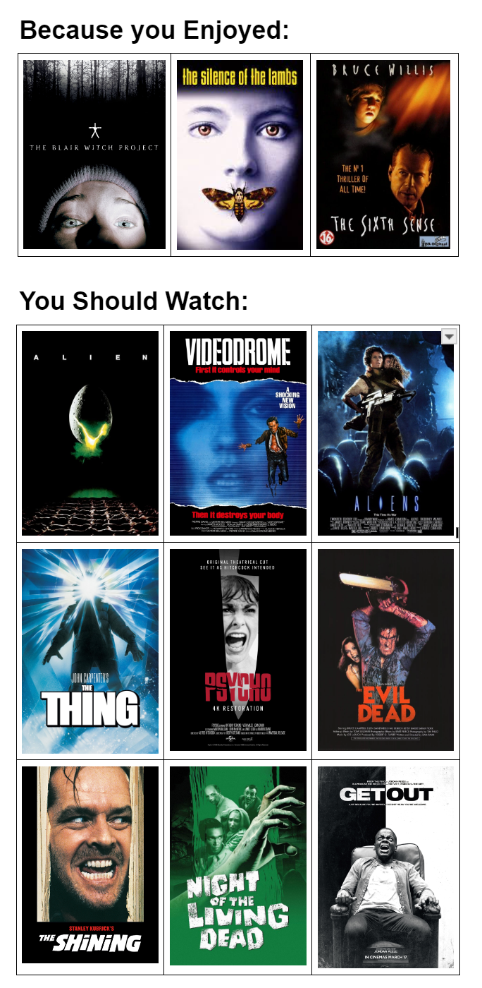
Horror Lover
Hello, Horror Lover
Because you like: [Horror]
And hate: [Children]

And enjoyed these movies:
Blair Witch Project, The (1999)
Silence of the Lambs, The (1991)
Sixth Sense, The (1999)

You should watch:
Alien (1979)
Videodrome (1983)
Thing, The (1982)
Aliens (1986)
Psycho (1960)
Evil Dead, The (1981)
Shining, The (1980)
Night of the Living Dead (1968)
Invasion of the Body Snatchers (1956)
Get Out (2017)
Children’s Movie Lover
Hello, Children's Movie Lover
Because you like: [Children]
And hate: [Horror,Romance,Drama]

And enjoyed these movies:
Toy Story 2 (1999)
Finding Nemo (2003)
Monsters, Inc. (2001)

You should watch:
Zootopia (2016)
Kung Fu Panda 2 (2011)
Incredibles, The (2004)
Madagascar: Escape 2 Africa (2008)
Kung Fu Panda (2008)
Bolt (2008)
The Lego Movie (2014)
Megamind (2010)
Rango (2011)
Goonies, The (1985)
Sci-Fi Lover
Hello, Sci-Fi Lover
Because you like: [Sci-Fi]
And hate: [Romance,Children]

And enjoyed these movies:
Star Wars: Episode V - The Empire Strikes Back (1980)
Matrix, The (1999)
Terminator, The (1984)

You should watch:
Spider-Man: Into the Spider-Verse (2018)
Blade Runner (1982)
Aliens (1986)
Star Wars: Episode IV - A New Hope (1977)
Nausicaä of the Valley of the Wind (Kaze no tani no Naushika) (1984)
Akira (1988)
Alien (1979)
Thing, The (1982)
Inception (2010)
Cowboy Bebop: The Movie (Cowboy Bebop: Tengoku no Tobira) (2001)
Comedy Lover
Hello, Comedy Lover
Because you like: [Comedy]
And hate: [Children]

And enjoyed these movies:
American Pie (1999)
Dumb & Dumber (Dumb and Dumber) (1994)
Austin Powers: The Spy Who Shagged Me (1999)
Big Lebowski, The (1998)

You should watch:
Sting, The (1973)
Thin Man, The (1934)
Kung Fu Hustle (Gong fu) (2004)
Some Like It Hot (1959)
Snatch (2000)
Midnight Run (1988)
What We Do in the Shadows (2014)
Office Space (1999)
21 Jump Street (2012)
Legend of Drunken Master, The (Jui kuen II) (1994)
Fantasy Lover
Hello, Fantasy Lover
Because you like: [Fantasy]
And hate: [Horror,Children]

And enjoyed these movies:
Lord of the Rings: The Fellowship of the Ring, The (2001)
Gladiator (2000)
300 (2007)

You should watch:
Princess Bride, The (1987)
Lord of the Rings: The Return of the King, The (2003)
Lord of the Rings: The Two Towers, The (2002)
Spirited Away (Sen to Chihiro no kamikakushi) (2001)
Monty Python and the Holy Grail (1975)
Yojimbo (1961)
Wings of Desire (Himmel über Berlin, Der) (1987)
Seven Samurai (Shichinin no samurai) (1954)
Star Wars: Episode IV - A New Hope (1977)
Raiders of the Lost Ark (Indiana Jones and the Raiders of the Lost Ark) (1981)
Romance Lover
Hello, Romance Lover
Because you like: [Romance]
And hate: [Children,Horror]

And enjoyed these movies:
Shakespeare in Love (1998)
There's Something About Mary (1998)
Sense and Sensibility (1995)

You should watch:
Life Is Beautiful (La Vita è bella) (1997)
Casablanca (1942)
Roman Holiday (1953)
Shawshank Redemption, The (1994)
Singin' in the Rain (1952)
Rebecca (1940)
Good Will Hunting (1997)
Forrest Gump (1994)
Pride & Prejudice (2005)
Modern Times (1936)
War Movie Lover
Hello, War Movie Lover
Because you like: [War]
And hate: [Children]

And enjoyed these movies:
Saving Private Ryan (1998)
Apocalypse Now (1979)
Full Metal Jacket (1987)

You should watch:
Schindler's List (1993)
Shawshank Redemption, The (1994)
Boot, Das (Boat, The) (1981)
Godfather, The (1972)
Dr. Strangelove or: How I Learned to Stop Worrying and Love the Bomb (1964)
Grave of the Fireflies (Hotaru no haka) (1988)
Great Dictator, The (1940)
Ran (1985)
Pulp Fiction (1994)
Lawrence of Arabia (1962)
Anti-Recommendations
What are the WORST movies for certain types of users? Do we get their least favorite genres?
To get anti-recommendations, we just print the bottom 10 (lowest predicted score) recommendations.
Children’s Movie Lover - Anti Recs
Hilariously, among the worst movies for someone who likes Children’s Movies, hates Horror and Romance, are Twilight and Nightmare on Elm Street. Those are definitely the worst possible movies for this user.
Hello, Children's Movie Lover
Because you like: [Children]
And hate: [Horror,Romance,Drama]

And enjoyed these movies:
Toy Story 2 (1999)
Finding Nemo (2003)
Monsters, Inc. (2001)

You should NOT watch:
Twilight Saga: New Moon, The (2009)
Legends of the Fall (1994)
Twilight (2008)
Boxing Helena (1993)
Lost Highway (1997)
Wolf (1994)
Bodyguard, The (1992)
Amityville Horror, The (1979)
Wes Craven's New Nightmare (Nightmare on Elm Street Part 7: Freddy's Finale, A) (1994)
Mulholland Drive (2001)
Horor Movie Lover - Worst Recs
For someone who loves Horror and hates Children’s movies, recommending Home Alone 3, Karate Kid, Free Willy, and Happy Feet are delightfully bad recommendations.
Hello, Horror Lover
Because you like: [Horror]
And hate: [Children]

And enjoyed these movies:
Blair Witch Project, The (1999)
Silence of the Lambs, The (1991)
Sixth Sense, The (1999)

You should NOT watch:
Inspector Gadget (1999)
Next Karate Kid, The (1994)
Home Alone 3 (1997)
Free Willy 2: The Adventure Home (1995)
Pocahontas (1995)
Super Mario Bros. (1993)
Happy Feet (2006)
Free Willy (1993)
Karate Kid, Part III, The (1989)
Honey, I Blew Up the Kid (1992)
Possible Improvements
Below are some possible ways to improve this current movie recommendation system:
- Add better movie features
- Use the movie’s year from the title as a feature (some people might like movies from certain eras)
- Use the movie’s title as a bag of words feature (helps model find similar movies based on title)
- Find and use the movie’s director/publisher (helps the model find similar movies based on who made them)
- Find and use the movie’s actors (some people have favorite actors)
- Leverage MovieLen’s ‘movie tags’ (requires lot of preprocessing but could be useful)
- Add better user features
- Find and use the user’s demographic features
- Leverage MovieLen’s user occupation feature (only available for some datasets)
- Use the user’s favorite ‘decade’ as a kind of genre feature (would work well if we added movie’s decade-year)
- Use the user’s favorite directors
- Use the user’s favorire actors
- Generate true training examples using the ratings timestamps
- Instead of randomly picking some movies to predict rating for, we can always use the last movies watched by the user as the labels and their earliest movie watches as their watch history
- Add an attention/context component to the model [ADVANCED]
- Transformers are all the rage, and because users have an order in how they watched movies, we could use them.
- Add movie reviews from IMDB or Rotten Tomatoes as text or sentiment features [ADVANCED]
- Reviews contain rich information about movies and also sentiment about if they are good or bad (in aggregate)
- Build a Deeper model
- This model is only one non-linear layer per input. We could go much deeper, ever after combining both user and item embeddings.
- Improve the model
- Add BatchNorm, Dropout
Appendix
Visualizing Movies in 2D
plt.figure(figsize=(15,15))
for movieId in top_movies[0:25]:
  i = item_emb_movieId_to_i[movieId]
  plt.scatter(ITEM_EMBEDDING_LOOKUP[i,0].data, ITEM_EMBEDDING_LOOKUP[i,1].data, s=200)
  plt.text(ITEM_EMBEDDING_LOOKUP[i,0].item(), ITEM_EMBEDDING_LOOKUP[i,1].item(), movieId_to_title[movieId][0:20], ha="center", va="center", color='black')
plt.grid('minor')
Example Training Runs
Below we will train the model on different datasets and with different model parameters.
| Dataset | Model Size | Observation | Loss Plot |
|---|---|---|---|
| Small | Small | Overfitting | 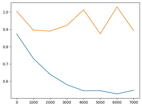 |
| Small | Medium | Extreme Overfitting | 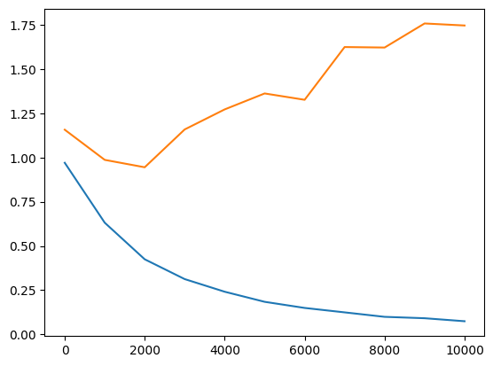 |
| Medium | Small | Loss is not great. Could keep learning but probably not worth it | |
| Medium | Medium | Training loss getting better but slight overfitting | 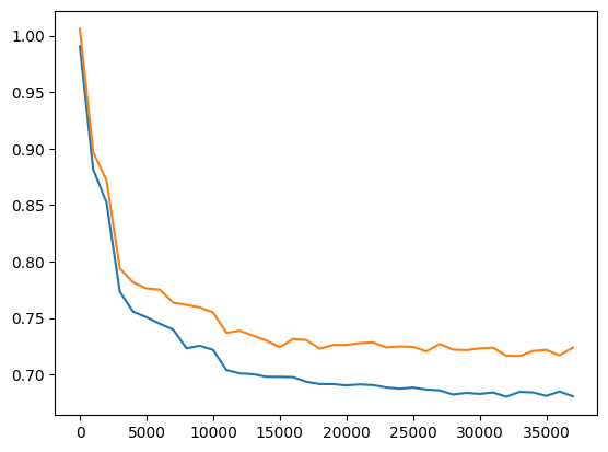 |
| Medium | Large | same as above | 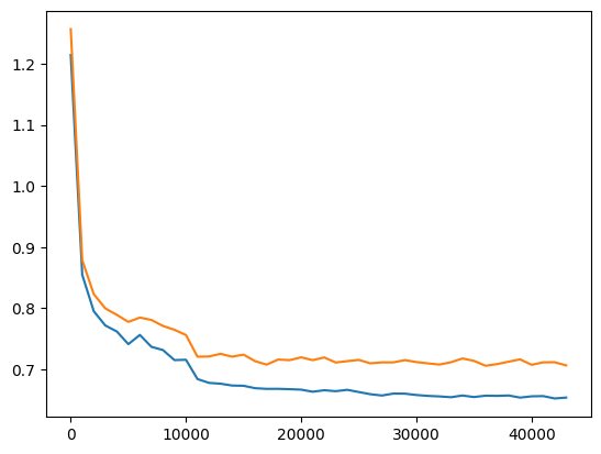 |
| Large | Small | No overfitting, but not learning well | 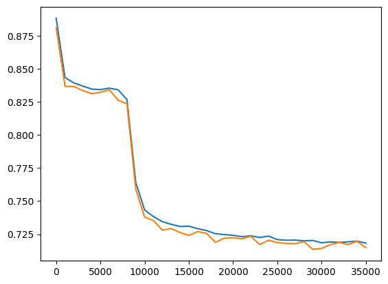 |
| Large | Medium | No overfitting, but hitting a wall | 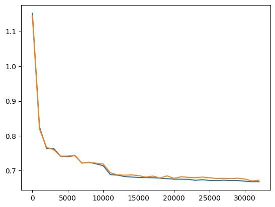 |
| Large | Large | Looking much better. Loss much lower than pervious runs | 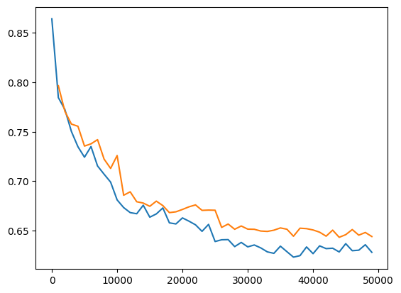 |
Applying Recommendations to Other Domains
NOTE: The below user/item features might be subpar for some domains. These ideas are how I would approach recommending items in each domain as a start. If you want more advanced descriptions, companies usually post techincal blogs about how they recommend content.
| Domain | User Features | Item Features |
|---|---|---|
| Online Shopping | Purchases Returns (negative signal) Reviews/Ratings Favorite Categories Country/City/State Yearly Purchase Count Yearly Purchase USD |
Brand Title Price Category Reviews Number of Returns |
| Books | Liked/Disliked Books Liked/Disliked Genres Liked/Disliked Authors |
Title Genres Book text (bag of words) Published Year |
| Music Streaming | Listened to Songs (with counts) Listened to Artists (with counts) Favorite Genres Time of Day of Listens Day of week of listens Country/State/City Language |
Title Genre Artist Listens Release Date ADVANCED: Embedding of Audio File |
| Social Media | Liked Posts Posts with > X seconds hover Following Account Ids Followers Account Ids Country/State/City Language Comments |
Account Id Bag of Words of Text/Caption Views per hour Likes Comments Comments Text ADVANCED Embedding of Image |
| Hotel Bookings | Past Bookings: Location Past Bookings: Hotel Favorite Hotel Brands Favorite Amenities Location Booking Count Viewed/Clicked Locations Viewed/Clicked Hotels Country Language Bookings in past year USD Spend in past year |
Location Brand Price Stars Reviews Amenities |
| Ads | Ad Purchase History Ad Click History Ad Spend USD last year Favorite Brands Country/City/State Age Gender Dependent on site serving the ads: Interests Page Clicks Searches |
Brand Product Categories Product Price(s) Clicks Click thru Rate Purchases Impressions Long Views |